Wave functions
[Note: This is a six section storyline. Starting anywhere other than section I, may cause confusion]
In classical mechanics, we consider the equations of motion of objects with definite positions and velocities. Big, classical objects work that way.
When we break those classical objects into their smallest components, elementary particles, we find that they don’t work that way. We can no longer imagine some definitively placed dot moving around in space and time.
An elementary particle is actually a wave. A wave made of what? That’s hard to explain upfront, but for an overly simplified start, let’s say probabilities - it’s a probability wave. Tabling the idea of momentum for a moment, it’s an object which is defined not by a definite position in space, but instead by a set of probabilities, one for every single position in space. It’s an infinitely expansive probability distribution for being in different positions, which itself, is shaped like a wave and evolves like a wave.
And we really mean all of space. Every single thing that you see around you (mind you that’s not much considering the billions of galaxies that are out there) is made of a virtually incomprehensible number of infinitesimally small particles, each of which having a probability for being everywhere in space, at once.
Weird. Why is it that large classical objects, like chairs and tables, look to be in a particular position at any given time? Recall that classical objects are made of tons of elementary particles, and at this scale, the underlying quantum characteristics average out. What’s more, they are made of a certain variety, of quantum wave function, which we will explore later (the fun world of bound states and coherent states - wave functions which have their probabilities bunched up around a relatively small area of space).
Classically, it’s as if objects have 100% of their probability sitting in one position and 0% chance of being anywhere else in space. You have the luxury of dealing with equations of motion that are rooted in evolving forward in time, definite states. In quantum mechanics, we can’t time shift, or evolve forward in time, definite states. We time shift or evolve forward in time, probability waves. And in the same way our wave function is defined by having probabilities for being in different locations, it also has probabilities for having different velocities (or momenta), vs. a single defined velocity. What’s more, the derivatives in our equations of motion are truly operational. They are concrete actions on concrete quantum mechanical wave functions. They actually shift waves around in space and time.
“Anyway, waves and particles are somehow the same thing, and if you want to penetrate that more deeply you got to learn some quantum mechanics. And a place to do it is in my lectures which don't cost anything, they're on the internet.”
Leonard Susskind | New Revolutions in Particle Physics: The Basics Lecture 1, ~46m | Stanford, YouTube
So we have two things to unpack. First, the wave function itself and this tricky idea of probability. That will be this section.
Second, operations on the wave function, which will be the two subsequent sections. Section 5 Symmetry Operators covers space translations, time translations, and space rotations - those three symmetries concern shifts of the wave function in real space. Section 6 Gauge Symmetries covers U(1) rotations, SU(2) rotations, and SU(3) rotations - those three symmetries concern shifts in tiny wrapped up spaces that you can't see.
Overview of this section:
Basic wave equation | It’s helpful to see the structure of a basic wave equation before jumping into quantum mechanics.
Probabilities | Explore the notion of probability in a simplistic way, and layer on the phenomenon of wave interference.
Prove it | Unpack the double-slit experiment, which brings out the phenomenon of wave interference and leveraged to prove whether something is a wave or not.
Complex numbers | Strictly speaking, the wave function outputs complex numbers called probability amplitudes, not real numbers. That complex number squared, is the real probability. To keep things simple before the complex number spiel, we will abuse language and call amplitudes, probabilities.
Basic wave equation
A wave wiggles. It wiggles around in space and time -or- it gets translated in space and in time -or- it gets operated on by space and time translation operators in the case of our quantum mechanical wave function. It exhibits both spatial and temporal variation, and there’s a differential equation, a differential wave equation to be exact, that relates its spatial variation to its temporal variation, i.e. its momentum to its energy. Schrodinger’s equation and Dirac’s equation are examples.
A particle is a solution to a particular differential wave equation. Solutions to differential equations, are functions. Solutions to differential wave equations, are wave functions. Fermions, quarks, electrons, and neutrinos, are wave functions that solve or satisfy the Dirac wave equation, for instance. Solutions to the Dirac equation are actually a little more complicated than a single component wave function, but we'll get to more complicated objects like spinors in the last section. Beforehand, we will find ourselves talking about waves generally and the simple model particle or plane wave e^i(kx-wt). It is a function of "x" and "t", or spatial position and time. "k" is the wave number or the spatial frequency of the wave and "w" is the temporal frequency of the wave.
Differential equations are built out of the derivatives of a function, which concern how the function's value changes or varies across the input space. Derivatives in operational uniform, are transformations that act on a function and do stuff to it, like shift it over in space or shift it over in time. The action of these symmetry operators leave properties about the plane wave invariant as they act. Space translation leaves invariant the wave's wave number or spatial frequency (inverse wavelength), and time translation leaves invariant the wave's temporal frequency. These are the symmetries that we use to build our simple differential wave equation, which relates the temporal variation of a wave to its spatial variation, or its frequency to its wave number, or its energy to its momentum.

Before we discuss the more complicated wave functions that roll up to classical physics, we will dissect the plane wave - it’s the simplest wave function and helpful to leverage in understanding the basics. Elementary particles like quarks are more complicated objects.
The video below will give you better feel for wave equations. It uses cos(kx-wt), though it is worth noting that cos(kx-wt), sin(kx - wt), and e^i(kx-wt) are very, very similar. Strictly speaking, sin is just shifted over a bit as compared to cos, and we use the complex exponential function when the wave is moving on a circle.

"A solution to the 2-d wave equation" | Wikipedia | Author: BrentHFoster
Probabilities
“So it became clear that light is made of indivisible elements called photons and that the wave character of the light really represents, or the wave pattern, really represents the probability that the photon appears at different places. (They) randomly arrive in blips, but arrive with a probability at different locations which follows the pattern that was established by the wave theory. The wave theory gives you a wave theory of probabilities. That’s quantum mechanics.”
Leonard Susskind | New Revolutions In Particle Physics: The Basics Lecture 1, 45m 42s | Stanford, YouTube
“So what is H (the Hamiltonian)? It's a rule for how you update the system. (If you) know it at an instant of time (you can) make an incremental change in the state of the system proportional to -iH times ψ. It’s a little machine for telling you how to update the system. Sounds awfully deterministic. But this one is not deterministic. Knowledge of the state of the system does not mean you know the outcome of every experiment. The state of the system tells you probabilities. This is a rule for updating probabilities. It evolves in a known and definite way. This is true if you do not interfere with the system. Interfere (and) you can disturb the system and change how it is evolving. Above is an undisturbed system that is not being measured. Measure something, disturb something else. Schrodinger wrote it for the motion of a particle. The generalized form can be applied to any system.”
Leonard Susskind | The Theoretical Minimum Lecture 5, 23m 46s | Stanford, YouTube
You are a classical object. If you stand in the middle of the street or anywhere else in space, you are definitely at a certain place. If you were somehow a quantum object, your state would change from being definitely somewhere, to being probably at some places and probably not at other places. It’s like "quantum you" is everywhere at once, but more of you is allocated to certain places rather than others. That is not exactly correct, but it helps with the intuition. It's hard to talk about quantum stuff with classical words. Keep in mind, we will also be avoiding the probability and probability amplitude distinction for a bit.
Let's limit "quantum you" to only three definite positions: In the middle, to the left, and to the right. The "classical you" was say, in the middle. Now we morph "classical you" in the middle, into "quantum you", a kind of probability pack across space that houses a probability for each available position. We get 100% to divvy up, as probabilities must always add up to 100%.

We take the set of definite states, to the left, in the middle, and to the right, and hit all three of them with probability weights. Our classical situation was comparable to shoving all of our probability into middle. Now we’re diluting the middle’s cut of the pie and spreading the love. Call that spreading, superposing. We assign probability weights to states and sum them up. We add and combine definite states, while properly diluting the probability for each state to ensure a total probability of 100%.
“You have to remember that in quantum mechanics, unlike classical mechanics, you get to add states. States form a linear, I'm going to say it, a linear vector space. That only means that you can add them, subtract them, and multiply them by ordinary numbers.”
Leonard Susskind | New Revolutions In Particle Physics: The Basics Lecture 3, ~38m | Stanford, YouTube
Classically, we don’t see things in more than one place, at one time.
If we look at "quantum you" at an instant of time, we will only see you in one of the three spots. Yes you are this probability distribution over space, but we classical objects can’t access this trippy space, called Hilbert space. Imagine Hilbert space as sort of hovering over real space and projecting onto it. Each time we look at you, 100% gets dropped into one of the three potential slots, i.e. we definitely see you somewhere, but sometimes you'd be in the middle, sometimes to the left, and other times to the right. If we accumulate statistics over many trials, we would find you to the left roughly 22% of the time, in the middle roughly 60% of the time, and to the right roughly 18% of the time. Not exactly, but roughly. We run a lot of experiments to approximate the situation. If we imagine ourselves taking these snapshots of you very rapidly, a "classical us", would see an averaged "classical you", about in the middle.
This is why some physicists like to use the phrase "virtual realities". There is a space of probabilities for different happenings and classically we get a definite average. Real and tangible quantities in our macroscopic world, are actually the statistical averages of quantum possibilities. Think of running a lot of experiments more naturally as, lots of quantum particles interacting with each other. Classical objects, are made out of lots of quantum objects. The probabilistic effects go away when you average over the dynamics of many particles. At the smallest levels, "we" look at "you", still refers to quantum waves talking to quantum waves. The actual act of observation or measurement between two quantum waves boils down to a mathematical operation called the inner product. Two wave functions become tied together at the hip, or correlated, and one must update the probabilities with both particles in mind. We move onto discussing a single multi-particle wave function, instead of two separate single particle wave functions. This is also called entanglement. Vector spaces equipped with this operation are called inner product spaces.
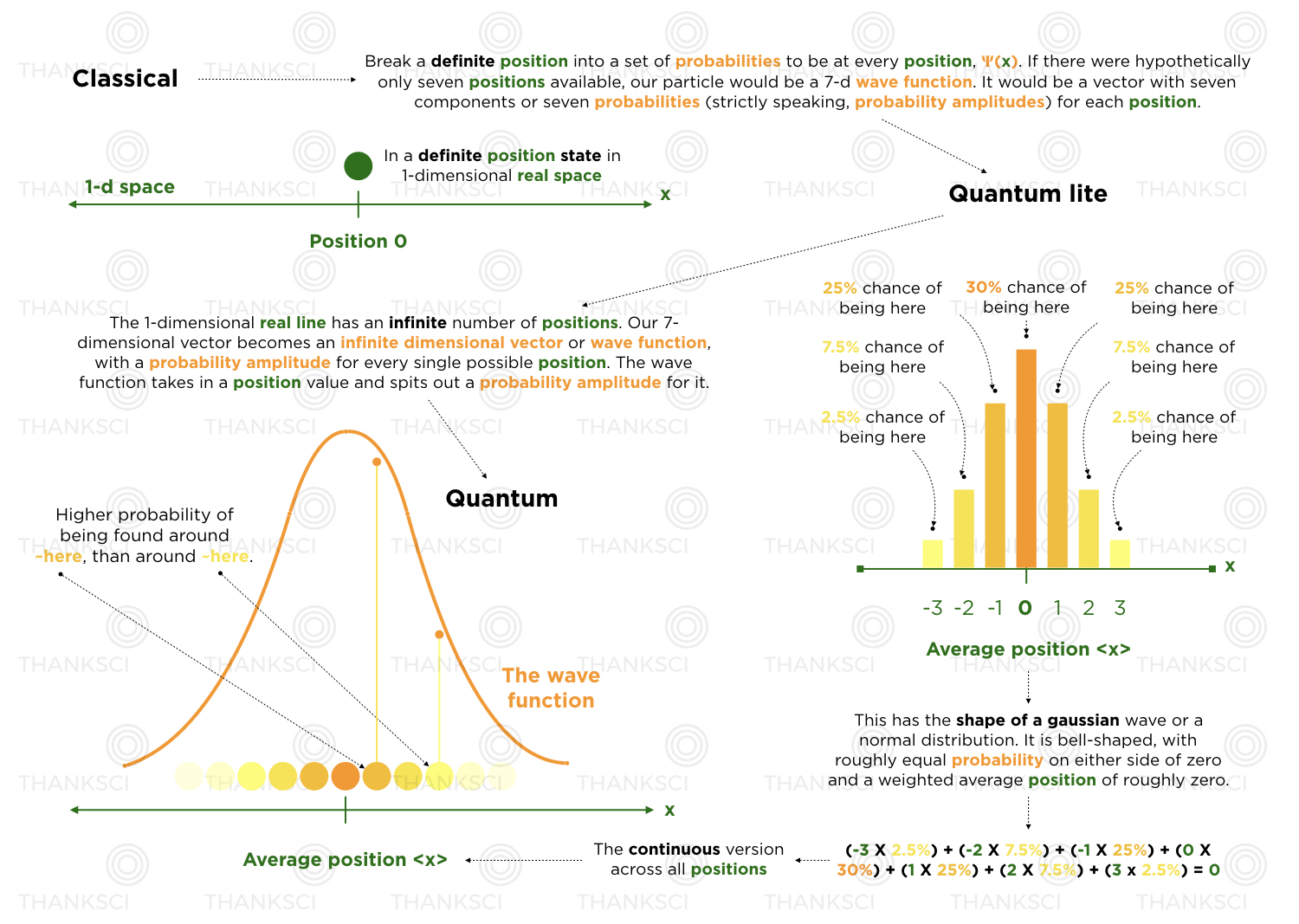
The wave we used in our diagram above, is called a gaussian. Its probability distribution pops up roughly around a position and virtually flat lines away from it. The wave defined over all of space, but its value is effectively zero outside of this neighborhood. We might even give our wave, with a reasonably well defined position, a little more personality.
.gif)

This wave has its probabilities bunched up around a certain spot, like the gaussian. Sure the wave function dips into negative territory some places, but remember, those become real, positive probabilities. Strictly speaking, the outputs of the wave function are probability amplitudes, which can be positive or negative, and the square of those amplitudes, are the probabilities. Input a position in space, output a probability amplitude. Square that for the probability. A positive peak and a negative valley of the same magnitude, represent the same real, positive probability.
The bunched up probability wave looks different from your standard plane wave. Our simple model particle, the plane wave, is spread out across space in a consistent and oscillatory fashion, with a constant wavelength. It doesn’t look different anywhere in space.
There are all kinds of waves… an infinite number of variations. Again, talking simplistic types like the simple plane wave allows us to work through important concepts in easy ways. The specific sort of category of wave functions we’ll ultimately be most interested in, the kind that rolls up to everything we see in classical physics, are called coherent states. More on those after the basics and the double-slit experiment.

This simple particle is equally likely to be everywhere. Discussing a nice, average classical position, makes little sense. Very different from the bunched up probability wave with a reasonably well defined position. The plane wave's wavelength however, is definite and constant. The wavelength speaks to how fast the wave wiggles. The plane wave has a definite velocity, or momentum.
There are two kinds of waves we will encounter. Any other wave is a mix between the two, and can lean more towards one extreme or the other. The extremes are essentially unattainable, but we can get close. There are waves with a terribly defined position but a well defined wavelength, and there are waves with a terribly defined wavelength, but a well defined position. This is a tradeoff with waves, either they have a nice position or a nice wavelength.
The wave with a perfect position, doesn’t look like a wave at all. It’s called a Dirac delta function. It is an infinitely tall and narrow spike at a particular point. It's basically like dropping 100% of our probability into one specific location. The other wave is our plane wave of perfect wavelength.

Consider that we can add waves, or superpose them, as long as probability adds up to 100%. That’s this whole "linear vector space" stuff. You can make a wave with a nice position, by adding together waves with a nice wavelength, and you can make a wave with a nice wavelength, by adding together waves with a nice position. We did a baby version of this earlier and you didn’t realize it. We took three definite position states (we would need an infinite number to make a plane wave), hit them with probability weights, and made a state which was a linear superposition of the three definite position states. Definite positions are like Dirac delta functions. This statement will make more sense in the next section, but one might say that the Dirac delta function is the eigenvector of the position operator.
We can also go the reverse direction. We can think of the plane wave as the definite state. Not a definite position state, but a definite wavelength state. We can take a ton of plane waves, hit those with probability weights, and make a state which is in a linear superposition of different wavelengths. We can actually represent the Dirac delta function, as a sum of plane waves. That's a very deep fact. Our discussion will tend to use the vantage point of stacking plane waves, which represent our simplest particles, to create waves with better defined positions.

Graphic: Christine Daniloff
Again, the idea here is that, you can make any kind of wave function, even the kinds called coherent states that roll up to classical physics, by adding together plane waves of different varieties. One wave function, that is also, the combination of many plane waves.
This is the essence of the Fourier transform. Or harmonic analysis. Or superposition. We can represent any arbitrary wave function, even one with its probabilities bunched up around a particular spot, as a sum of plane waves. We can break a complicated wave up into simple pieces. The tradeoff between position and wavelength is called the uncertainty principle and is simply a statement about the Fourier transform. We can't have our cake and eat it too. We either have a wave with a more defined wavelength, or a wave with a more defined position, but not both.
A series of plane waves can make a wave with a reasonably well defined position, through interference. When waves are combined, they interfere and can do so either destructively or constructively. Although probabilities are always positive, the wave function takes on positive or negative probability amplitudes, and those get added before the probabilities are calculated. Check out this picture. The left side shows two waves whose peaks and valleys match up. They constructively interfere. They amplify each other. The right side of the picture shows two waves, where one wave’s peaks line up with the other wave’s valleys, and vice versa. Those two waves destructively interfere, or cancel each other. Where one is positively-valued, the other is negatively-valued.

"Interference of two waves" | Wikipedia | Authors: Haade, Wjh31, Quibik
If you find yourself combining plane waves of various wavelengths, and thus frequencies (there is a definite frequency that goes with a definite wavelength), the interference might be such that the probability is clumped up around a spot. It’s in a linear superposition of plane waves which are destructively interfering outside of this little area, and constructively interfering inside of this little area. FYI, classical limitations are still at play. We only get one frequency option with each individual measurement, and we accumulate statistics to get the average.

We are considering the shape of a probability distribution over space and how it evolves over time. It’s shaped like a wave. It evolves and oscillates like a wave. The probabilities, which are the wave outputs squared, add up to 100%.
Waves have certain properties: Amplitude, wavelength, and frequency. The output value or the height is one. That’s amplitude. That’s probability amplitude in quantum mechanics. The shape of the probability distribution varies across space. Wavelength speaks to the spatial variation. Shorter wavelength waves exhibit more variation across space. Finally, we have frequency. The probability distribution isn't stagnant. It evolves over time. It moves. It wiggles. It has spatial variation and temporal variation. Spatial variation = wave number which is inverse wavelength. Temporal variation = frequency which is inverse period. Period is just the time it takes for the wave to wiggle once. Shorter wavelength waves will have higher frequencies. Certain frequencies go with certain wavelengths. There is an equation which links them, called the differential wave equation motion. Sometimes it's called Schrödinger's equation. Sometimes it's called the Dirac equation. Sometimes more generally, it's called the Hamiltonian. High frequency, short wavelength waves wiggle very rapidly. Low frequency, long wavelength waves do not.
An object with its probabilities bunched up around a point has a shape which shows off a reasonably well defined position, but a poorly defined wavelength. The single wave can be considered to be a linear superposition of simpler plane waves which enjoy definite frequencies. There is uncertainty in the particle's position, but not as bad as a plane wave. Waves of definite wavelength travel with a definite velocity. Call it the phase velocity of the wave. Our bunched up probability wave however, is made of several waves with definite velocities, and travels at what is called, the group velocity. That sort of averages over the individual velocities underneath the hood.

There are two kinds of quantum waves, bosons and fermions. Bosons like to be in the same state. They like to be waves of the same wavelength and frequency that stack on top of each other. The group velocity and phase velocities like to match up. They like to form classical waves, or force fields. Light is a good example. Photons stack on top of each other to make classical light waves. Light travels absurdly fast. It's faster than anything in the universe. Position is a terrible attribute to use in describing a photon. Velocity however, is a great one.
Fermions can’t be in the same state. If we want to stack fermions on top of each other at the same place, we need waves of different momenta and frequencies. We can find ourselves with waves that have reasonably well defined positions.
Prove it
This sounds all fancy, but have we seen it? Yes. This is physicist tested and mother approved.
How do we prove anything is a wave? We look for evidence of interference. Waves interfere. In the lecture below, Susskind proves that all particles, both bosons and fermions, are waves. We’ll provide a quick rundown of the main points, but watch the lecture (~0m to ~51m) if you have the time.
New Revolutions in Particle Physics: Basic Concepts Lecture 1
Leonard Susskind | Stanford, YouTube
~0m - 22m | history of our exploring the question “is nature discrete or continuous?”, the discovery of atoms (John Dalton), Becquerel’s discovery of radioactivity (beta = negatively charged electrons, electrically neutral gamma = photon, positively charged alpha = helium)
~22m - 32m | the wave character of light, a qualitative discussion of the electromagnetic field, history of wave theory (brief), review of Thomas Young’s 1801 double slit experiment which proved the wave character of light (demonstrated that light waves exhibited the property of interference, a property specific to waves)
~32m - 41m | details of wave mathematics, wavelength (distance in space for a full wave cycle), period (time that it takes to complete a full wave cycle), the fundamental wave equation (the distance that it moves, or wavelength, divided by the time that it takes to move that distance, or period, equals the velocity of the wave) and the connection between wavelength and period (the longer the wavelength, the slower the period, the shorter the wavelength, the faster the period), frequency (inverse period, or number of oscillations or cycles per unit time), omega (still just frequency, but number of radians per unit time, 2π radians = 1 cycle)
~41m - 47m | the particle character of light and the quantization of light, brief history of light quantization (Einstein and Planck), experimental evidence of light both being made of individual discrete units (photons) and exhibiting wave properties (interference, dilute light version of double slit experiment), wave character coming from quantum mechanics and reflecting the little unit’s (the photon’s) likelihood to be in different places (wave of probabilities)
~47m - 51m | electrons as waves, the electron double slit experiment proving wave character (demonstrates interference), the double-slit experiment demonstrated with large objects (bucky balls, 60 carbons) and its potential use on larger and more interesting things (viruses)
Classical light is a wave. We can prove that light is a wave by doing something called a double-slit experiment. Roughly, you send a wave at a surface with two slit like openings in it, the wave propagates through both slits, and splits into two waves. Those two waves recombine on the other side and show off interference patterns.

"An illustration of the double-slit experiment in physics" | Wikipedia | Author: Johannes Kalliauer, Wikigraphists | Note: THANKSCI adjusted
As the two waves come back together, they constructively interfere in some places and destructively interfere in other places. Showing that something does this, is enough to say hey, that thing is a wave. Here’s what happens if you shine a flashlight onto a wall (below left). You get a blob. That doesn’t look like a wave. How can we test whether or not it is actually a wave? Shine your light through a double-slit (below right). Voila, we see that light is a wave. Why? The light splits into two waves, recombines, and amplifies some places and not in others. We get an interference pattern.


That was a classical interference experiment. Light waves are actually made of discrete little quantum mechanical pieces called photons. Each photon has a definite frequency and brings a certain discrete amount of energy to the fiesta. How can we see that? When we turn down the intensity on our classical light, so as to turn what was once a classical beam of light made of tons of photons, into a beam of light with far fewer photons, we start to see discrete blips of light hit the screen. If we shine our low intensity light at a double-slit, we will start to see discrete blips of light hit the screen, and show off an interference pattern.

What if we did this with fermions? Would we see any signs of interference? Indeed we would. Fermions are also waves. A single electron is not defined by a single position, but a probability to be at every single position in space. As real objects, we have to get at this pattern over time, with many trials. Real objects can’t see all the happenings of Hilbert space. We can only see one possibility at a time.
We send in electrons, one at a time. Each one, is a quantum wave function, which breaks into two, recombines, and shows off an interference pattern. The screen, which all of our electrons hit, measures our electrons. Before an electron hits the screen, it is essentially a probability distribution over space, and after it hits the screen at a particular location, all of the probability from outside of that impact location, gets scooped up and dropped off into that impact location. The screen observes the electron at that spot. Again, an electron wave comes in, interferes with itself, shakes up the probabilities to be concentrated along one of the constructive interference bands, and once the electron hits the screen, it picks somewhere to be, but based on the probability function it had right before impact.
If we were to keep shooting in electrons, what might we expect? We’d expect all of our electrons to do the same thing and continue, not to choose exactly where they will land, but interfere with themselves such that they find themselves likely to be along one of the bands. We'd expect them to start filling in the bands and showing off the interference pattern, over time.


"Particle impacts make visible the interference pattern of waves" | Wikipedia | Author: Thierry Dugnolle
“There’s a connection between waves of any kind, and particles. They are not two different things. Somehow, waves and particles are two manifestations of the same thing. Waves and particles, at least when it came to light, were somehow intimately connected. It didn’t make sense to say light is a particle, or it didn’t make sense to say light is a wave, but it has manifestations of both. Alright, the situation only got more complicated when electrons were studied. Electrons are clearly particles. Everybody knows electrons are particles. There was no ambiguity about that, no more ambiguity than there was about whether light was a wave or not. Well something funny also happened with electrons. You could do exactly the same kind of experiment with electrons as you can (with photons). Today this experiment can really be done. At the time it was a bit of a thought experiment but equivalent. You have to put the holes, you have to make a screen… you put the holes, much closer to each other if you want to do with electrons, for one reason or another… and you send electrons through. Of course they come through one at a time. Everybody knew electrons were little particles that came through one at a time but was totally unexpected is, or would have been unexpected was, that the electrons, when you open two holes, form an interference pattern. In wasn't just that light was funny. Particles were funny in general. Our electrons exhibited wave properties, light exhibited particle properties. In fact, had we taken the alpha particles, which are much heavier than electrons, 8,000 times heavier than an electron… much harder to do these kind of experiments with, but send them through two little holes like that we also would see interference patterns. This has been done with objects which are much bigger than helium nuclei namely bucky balls. Bucky balls have been sent through and seen to form the same kind of interference pattern. Everybody know what a bucky ball is? 60 carbons. 60 in a shape of a generalized soccer ball.”
Leonard Susskind | New Revolutions In Particle Physics Lecture 1, ~47m | Stanford, YouTube
The wave functions we care most about, are the ones which are trapped. An electron wave function trapped in rotation around a nucleus, is called a bound state. It gets bounded to the nucleus, because it starts tossing a photon back and forth with it. The photon is in a quantum linear superposition of being attached to both. Atoms bind together by tossing electrons back and forth. Or in quantum speak, an electron can be in a superposition of being around one nucleus, and another nucleus. In chemistry speak, the two atoms share an electron or form a covalent bond.
The ground state electron wave function in the hydrogen atom, nature’s simplest atom formed by just a single electron and a single proton, is roughly around a particular place and roughly has a defined frequency. We are having our cake and eating it too, to the largest extent possible. It makes for a nice approximate situation, but still has the undeniable uncertainty we expect from waves. Sometimes we call it a minimum uncertainty state or a coherent state. Bound states lead to discrete energy levels and all of classical physics. No bound states, no classical physics. Don’t get too confused here, we will bite into this cookie in subsequent sections with a more group theoretic twist: The electron here, is a 3-dimensional wave function, called a spherical harmonic, that is rotationally symmetric and transforms as a representation of the special orthogonal group SO(3), or the group of 3-dimensional rotations.

"Visual representations of the first few real spherical harmonics" | Wikipedia | Author: Inigo.quilez

"Atomic orbitals of the electron in a hydrogen atom at different energy levels" | Wikipedia | Author: PoorLeno | Note: The probability of finding the electron is given by the color, as shown in the key at upper right.

"A wave function for a single electron on 5d atomic orbital of a hydrogen atom" | Wikipedia | Author: Geek3 | Note: The solid body shows the places where the electron's probability density is above a certain value (here 0.02 nm−3): this is calculated from the probability amplitude. The hue on the colored surface shows the complex phase of the wave function.

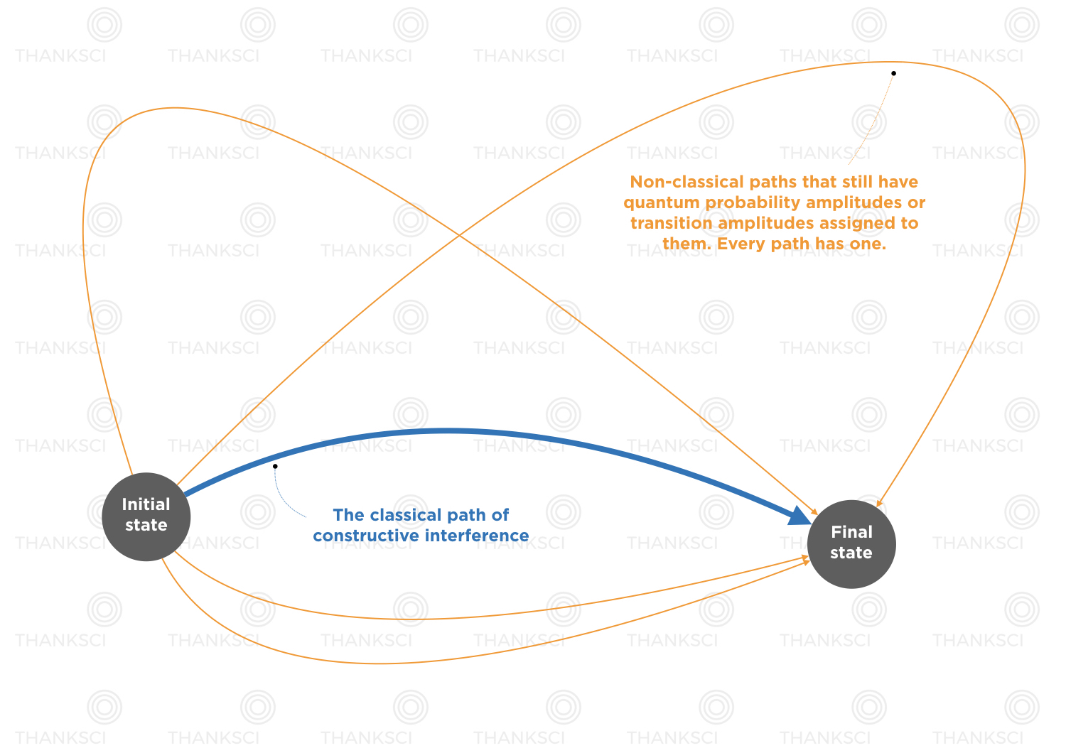
Nature really is quantum mechanical. How might this change our view of the classical trajectory from classical mechanics? There we explored how a particle’s position (and velocity) changes. Now we’re saying that the particle is not in any one place, for sure. Your equation of motion still tells you how to update your system, or evolve things forward in time, but now it tells you how to evolve forward the probabilities for situations to occur, not definite situations. Classical physics is deterministic. Quantum physics has undeniable uncertainty. Trajectories are assigned probability amplitudes and what technically occurs quantum mechanically, is a superposition of all possible trajectories. The trajectories which constructively interfere, end up being the trajectories that, conserve energy and momentum, are most probable, and ultimately shake out to be something classical. This gets covered in the path integral formulation of quantum mechanics.
“They tend to cancel a lot. The only trajectories which tend not to cancel, are the ones near the classical trajectory. We don’t have to discuss that now, but that is the way you go from quantum mechanics to a classical theory, at least in this formulation, if you look for the particular trajectories where you have the least cancellation, those are the trajectories of stationary action, where the action is minimum. But that’s another story. This is the quantum mechanical path integral formulation that much of modern field, basically all of modern field theory, quantum field theory, is based on.”
Leonard Susskind | New Revolutions in Particle Physics: The Basics Lecture 10, ~20m | Stanford, YouTube
Complex numbers
Strictly speaking, the wave function doesn’t output a probability, it outputs a probability amplitude. Probability amplitudes are complex numbers. Waves are complex functions. A function is a transformation. It maps an input to an output. The input of our wave function is a particular point in space, and the output is a complex number. The wave function is an infinite dimensional vector in that it boasts a probability amplitude for every position in space.
The real numbers form a mathematical structure. There are 1-dimensional real numbers. They sit on the real line. Think of the real line, as a geometry. It’s a continuous geometry with a definition of nearness between points.
The complex numbers form some other mathematical structure. You probably don't remember discussing these troublemakers in school. A complex number is more complicated than a real number. If a real number wanted to impersonate a complex number, it would need another real friend. It takes two real numbers to impersonate a 1-dimensional complex number. What's more, the complex numbers are also points on a geometry. Not a straight line though. This time, a circle.
What's even more, the two geometries are topologically equivalent, or you might say, naturally connected. There is a very special mathematical map that connects the two geometries. Our universe depends dearly on this map. The most important equation featuring this map was once called by Richard Feynman:
Euler's formula is ubiquitous in mathematics, physics, and engineering. The physicist Richard Feynman called the equation "our jewel" and "the most remarkable formula in mathematics".
"Euler's formula" | Wikipedia
This map allows us to represent complex numbers, in terms of real numbers. It connects the two structures. Euler’s formula shows off the connection. That’s good. We think in real numbers.
A complex number is represented as a function of two real numbers, r and θ (or a and b). r is the length of the arrow (the arrow which represents our complex number and points at a spot on a circle) and θ is the arrow's angle or phase (angular separation from the real line). θ ranges from 0 to 2π. As θ varies, we rotate around the circle. Once we hit 2π, we’re back where we started from. π is a real number. It’s a weird one though. It’s approximately 3.14. "e" is also a real number. It's approximately 2.71. "i" is a complex number that lines up with e^i(π/2). This function is called the complex exponential function. It allows us to represent 1-dimensional complex numbers with 2-dimensional real numbers.

The outputs of wave functions, are probability amplitudes, which are just complex numbers. Waves, are complex-valued functions. It's now no wonder that our plane wave, which takes on values over and oscillates over real space, has the form e^i(kx-wt), "x" being position in space, "t" being time, "k" being wave number (inverse wavelength) and "w" being frequency. We need the complex exponential function to bridge the geometric gap.

Now for perhaps the deepest fact about the complex exponential function. It is invariant under differentiation. Recall our interest in symmetry operators which act on wave functions and leave properties of those waves invariant. Our model particle or plane wave plays an important role in the concrete representation of certain abstract symmetry operators. In the next section, we will explore the plane wave’s invariance under space translations and time translations. Towards the end of that section, we'll explore rotations. We need those for bound states. In the final section, we'll complicate our wave function and throw in gauge transformations.
“If you have the real line. That is our set S. That is going to map, by the map "f is equal to e^i2πt (f=e^i2πt)", down to the circle, the complex numbers, (or) S1. The fibers of that map... if you look at all the points mapping to 1, those are the points 0, 1, 2, 3, -1, etc. This map is surjective. And the set of equivalence classes for this map, just consists of the interval 0 and 1, with the end points adjoined. f inverse of 1 is the collection of integers. Because any point has a preimage in there, that identifies the equivalence classes with the circle, because if you link up the two points of that interval you get a circle.
This is a fairly famous and complicated map of sets. The equivalence classes are the image. For each point in the image, you have a fiber above it, that’s the equivalence class containing it. Maps of sets are fairly complicated. We are going to apply this to maps of groups, where the situation is much nicer.
By the way, this is a map, or a homomorphism of groups. We have the additive group of real numbers, and the circle is the multiplicative group of numbers on the circle. Happens to be the fact that f(a+b) = f(a) + f(b). That’s the property of the exponential function, that it gives a group homomorphism. That’s why we study it. It is a group homomorphism. It is rather remarkable, the exponential function. First out of two amazing properties.
1. This f(a+b) = f(a)dotf(b) property. That it is a group homomorphism from the additive group to the multiplicative group.
2. But even more amazing than that, is that it is the solution to this differential equation: f’ = 2π(i)f
This is a differential equation that comes up often in math. You might think is there a relation between group homomorphisms and solutions of differential equations. When you go on to study the subject of Lie groups... which are not only groups, but continuous groups on topological spaces (lecturer points at the real line). This is not just a set, it has a topology on it (lecturer points at circle). You can say when two points are within an epsilon neighborhood of each other. And if you notice that this group homomorphism not only preserves the group structure, but sends points that are close up here (points at real line) to points that are close down here (points at circle). It also preserves the topological structure. This is a homomorphism of Lie groups.
And you are going to discover, this is one of the great discoveries by Sophus Lie at the end of the 19th century, that the study of group homomorphisms, in the context of continuous groups, is intimately related to the solutions to differential equations. Let’s talk about equivalence relations in the context of groups, which the exponential map is. We’re going to get one if we take a map of sets, which is a group homomorphism.”
Benedict Gross | Abstract Algebra Lecture 5, 8m 46s | Harvard, YouTube